Recent audio restoration increasingly relies on large-scale conditional latent generative modeling, including diffusion, Schrödinger Bridges, and Flow Matching variants, to invert degradations such as bandwidth limitation or noise. We present an analysis of the performance of various state-of-the-art methods compared to simple arithmetic transformations in the latent spaces of multiple neural codecs for musical bandwidth extension. We show that estimating a single transport vector between the clean and degraded latent centroids on a reference set, and adding it to degraded latents, can yield restoration performance competitive with large diffusion models. This suggests, first, that some neural codec latent spaces exhibit structure aligned with audio bandwidth; and second, that in such cases complex conditional models may offer only limited gains over a simple vector addition. We argue that these findings reveal an interesting avenue for future research whereby models could take advantage of the latent space structure in order to offer greater training and parameter efficiency, and overall better performance. Additionally, we propose to consider this simple arithmetic transformation as a baseline for music bandwidth extension research, as it allows an assessment of the contribution of learnable parameters towards restoration performance.
Paper Materials
Figures and tables from the manuscript are provided below, with expandable tables for compact browsing.
Figures
Figure
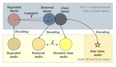
Conceptual restoration pipeline
We analyze audio restoration through latent transport geometry. For bandwidth extension, simple low-parameter latent transports already achieve strong waveform results on common audio metrics, in some cases approaching large generative baselines. For other degradations, the latent correction is less coherent, showing that restoration difficulty depends strongly on the encoder and the degradation.
Figure
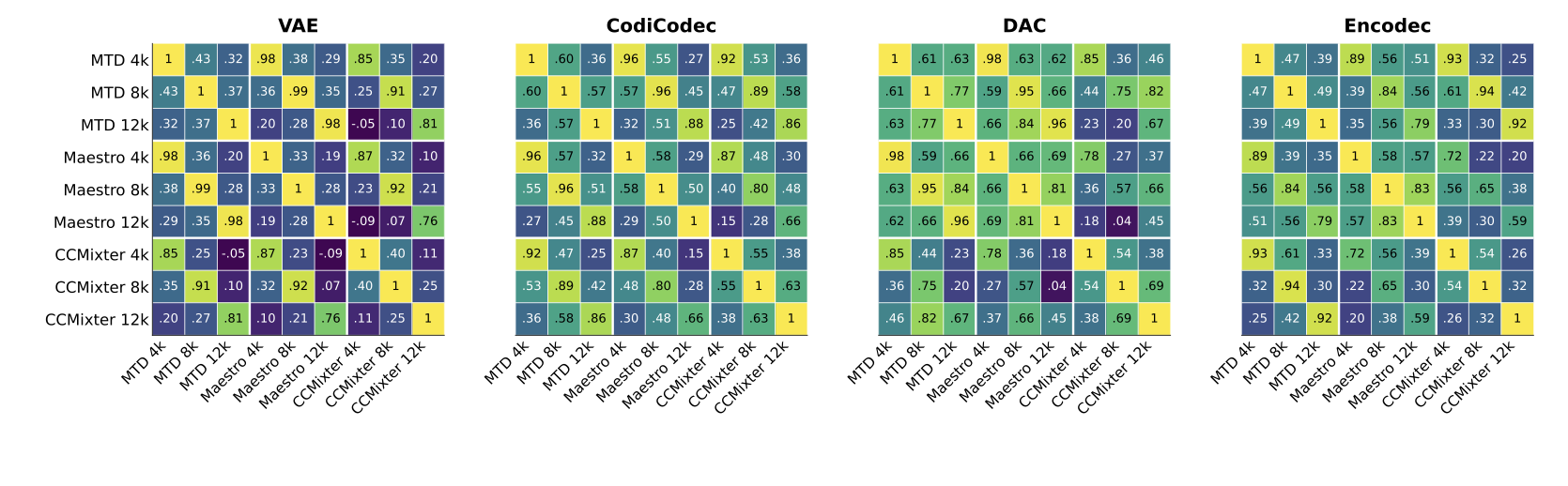
Cross-dataset consistency of latent BWE transport
Per-codec cosine-similarity heatmaps of global mean-shift transport vectors across all dataset-cutoff conditions for bandwidth extension. Each panel corresponds to one codec and compares the nine conditions formed by the three datasets (MTD, Maestro, and CCMixter) and three cutoff frequencies (4, 8, and 12 kHz).
Figure
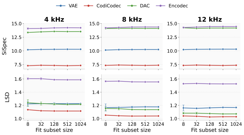
Sample efficiency of mean-shift estimation across codecs
Raw-clean SiSpec and raw-clean LSD as a function of fit subset size, grouped by cutoff and codec. Starting with just 8 samples, most curves remain nearly flat as the fit subset grows, suggesting strong sample efficiency for deriving useful transport probes.
Figure
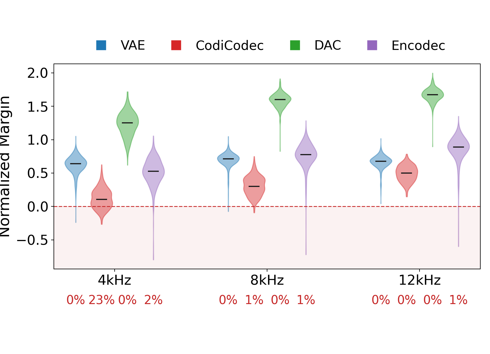
Identity preservation analysis across codecs
Normalized BWE margin violin plots across codecs and cutoffs. Percentages beneath each codec indicate the share of samples with negative normalized margin. Lower percentage means better identity preservation.
Tables
Table
Bandwidth extension results on MTD
Bandwidth extension results on mtd. Values match Table 2 in the manuscript and compare large learned baselines with zero-parameter mean-shift transports across VAE, CodiCodec, DAC, and Encodec.
Show table
Method
Variant
Parameters
4 kHz
8 kHz
12 kHz
LSD
SiSpec
ViSQOL
LSD
SiSpec
ViSQOL
LSD
SiSpec
ViSQOL
AudioSR†
±280M
1.75
21.74
3.39
1.81
27.26
3.23
1.85
28.97
3.15
CQTDiff†
±15M
1.74
10.62
1.75
1.63
17.42
1.78
1.57
21.62
2.00
IBAR†
±1B
1.12
12.31
2.99
0.92
12.94
3.52
0.85
13.08
3.84
A2SB†
no partitioning
±565M
1.33
25.51
2.55
1.05
33.10
3.20
0.87
35.34
3.93
2-partitioning
±565M
1.29
28.15
3.10
1.07
34.36
3.71
0.88
35.97
4.20
4-partitioning
±565M
1.77
27.56
3.44
1.59
34.25
3.82
1.51
36.07
4.27
VAE
mean shift
0
1.29
10.01
3.45
1.15
10.13
3.84
1.14
10.13
3.78
CodiCodec
mean shift
0
1.17
7.03
3.22
1.08
7.09
3.41
1.05
7.08
3.59
DAC
mean shift
0
1.23
13.37
3.14
1.15
13.98
3.54
1.08
14.10
3.85
Encodec
mean shift
0
1.64
8.10
2.31
1.59
11.07
3.18
1.55
11.21
3.57
Table
Bandwidth extension results on Maestro
Bandwidth extension results on maestro. Values match Table 1 in the manuscript and report cutoff-specific LSD and SiSpec for external baselines and mean-shift transports across all four codecs.
Show table
Method
Variant
4 kHz
8 kHz
12 kHz
LSD ↓
SiSpec ↑
LSD ↓
SiSpec ↑
LSD ↓
SiSpec ↑
CQTDiff†
1.154
31.49
1.137
32.99
1.129
33.33
IBAR†
0.769
12.69
0.688
12.22
0.616
13.48
A2SB†
4-part⋆
0.773
34.32
0.659
41.69
0.545
42.60
VAE
mean shift
1.185
11.34
1.164
11.34
1.130
11.36
CodiCodec
mean shift
0.975
7.94
0.938
7.97
0.923
7.91
DAC
mean shift
1.041
15.35
1.003
15.64
0.998
15.72
Encodec
mean shift
0.901
19.50
0.799
19.91
0.742
20.05
Table
Bandwidth extension results on CCMixter
Bandwidth extension results on ccmixter. Values match Table 3 in the manuscript and compare large learned baselines with zero-parameter mean-shift transports across VAE, CodiCodec, DAC, and Encodec.
Show table
Method
Variant
Parameters
4 kHz
8 kHz
12 kHz
LSD
SiSpec
ViSQOL
LSD
SiSpec
ViSQOL
LSD
SiSpec
ViSQOL
AudioSR†
±280M
2.00
12.50
2.74
1.86
14.93
3.09
1.75
18.35
3.51
CQTDiff†
±15M
2.01
14.67
1.97
2.06
15.88
1.86
2.10
16.34
1.85
IBAR†
±1B
1.64
7.11
2.37
1.41
10.46
2.60
1.36
7.86
2.74
A2SB†
no partitioning
±565M
1.93
14.05
2.77
1.71
19.95
3.20
1.48
27.17
4.04
2-partitioning
±565M
1.85
18.00
2.85
1.62
23.39
3.43
1.45
29.26
4.21
4-partitioning
±565M
1.84
17.46
2.65
1.65
23.17
3.43
1.50
29.20
4.23
VAE
mean shift
0
1.57
10.21
2.74
1.44
10.67
3.12
1.31
10.74
3.63
CodiCodec
mean shift
0
1.52
6.02
2.67
1.41
6.33
2.96
1.30
6.35
3.42
DAC
mean shift
0
1.71
12.03
2.65
1.56
12.88
2.90
1.51
13.45
3.58
Encodec
mean shift
0
1.92
18.22
2.72
1.83
18.72
2.93
1.73
18.93
3.49
Table
Restoration task complexity in latent spaces
Average cosine similarity and ΔLSD metrics on mtd across codecs using the global mean-shift transport. Values match Table 4 in the manuscript, where lower ΔLSD means more reduction and therefore more improvement in log-spectral distance.
Show table
Task
VAE
CodiCodec
DAC
Encodec
cos(θ) ↑
ΔLSD ↓
cos(θ) ↑
ΔLSD ↓
cos(θ) ↑
ΔLSD ↓
cos(θ) ↑
ΔLSD ↓
BWE
0.985
-2.086
0.986
-0.928
0.986
-2.286
0.481
-1.941
Denoising
0.627
-0.516
0.596
-0.502
0.596
-0.755
0.464
-0.540
Declipping
0.337
-0.002
0.290
-0.025
0.189
-0.069
0.129
+0.002
Dereverberation
0.295
-0.065
0.281
-0.228
0.323
-0.406
0.218
+0.158
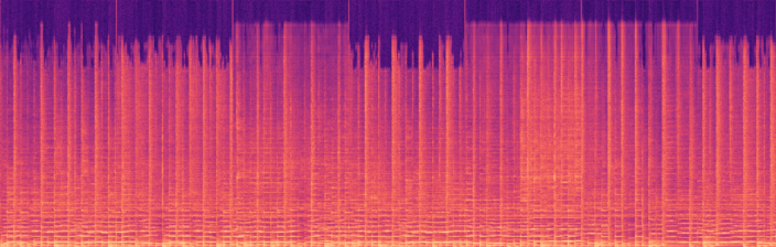
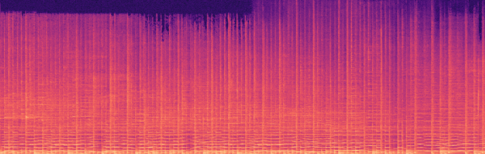
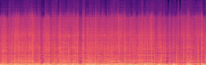
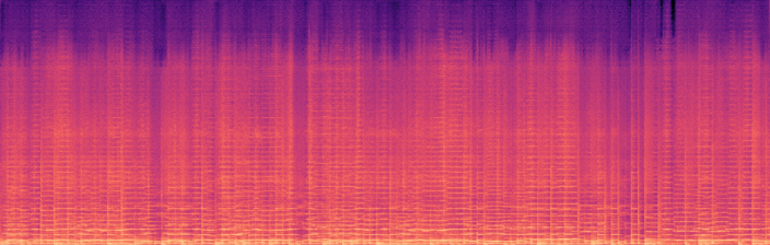
Comparison of Bandwidth Extension Baselines and Mean-Shift Latent Transports
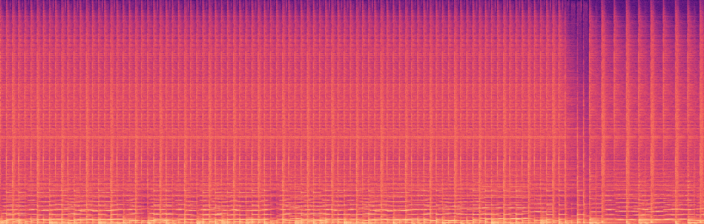
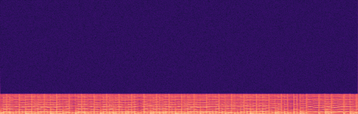
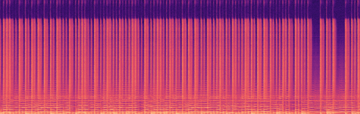
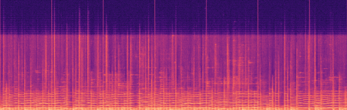
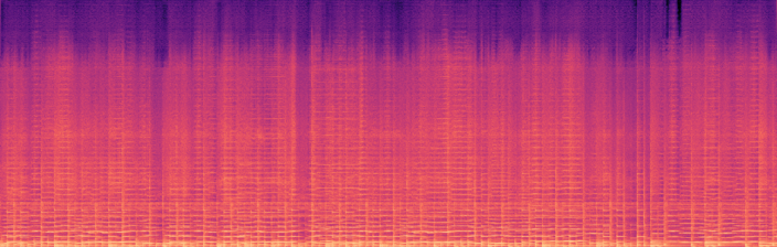
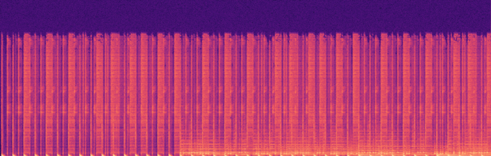
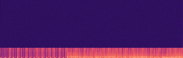
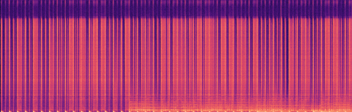
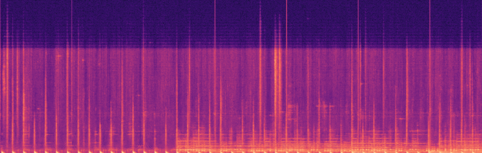
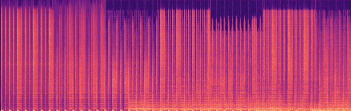
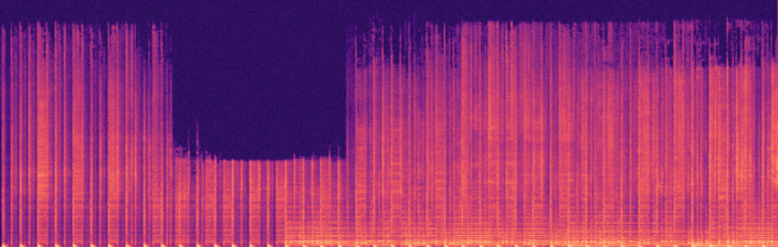
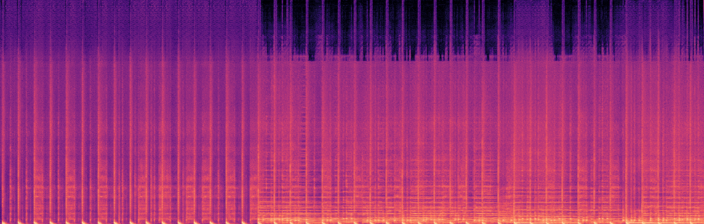
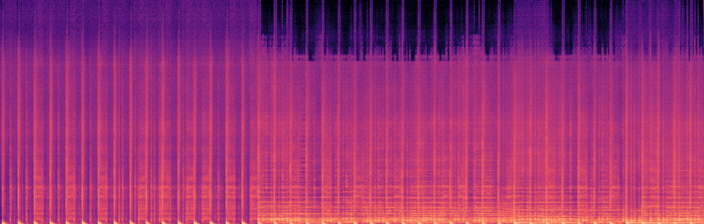
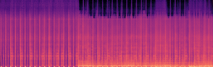
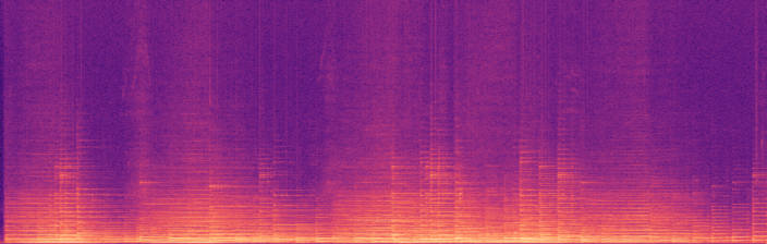
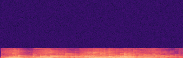
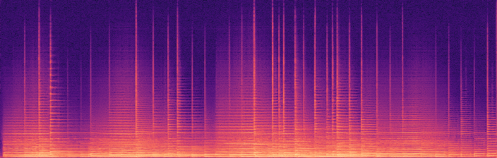
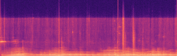
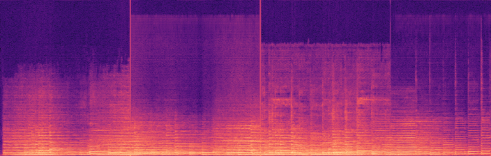
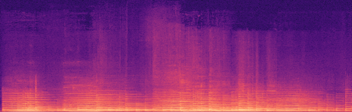
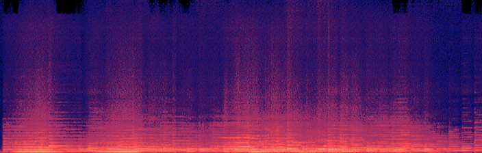
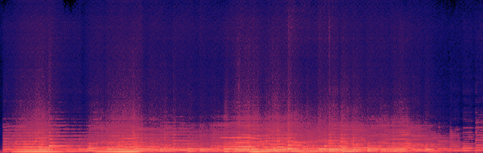
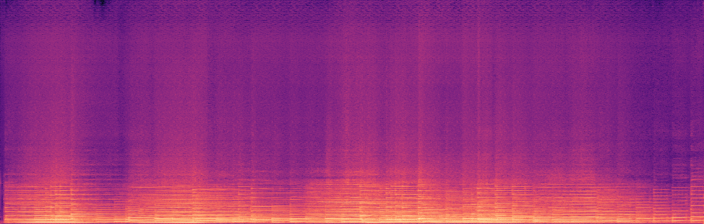
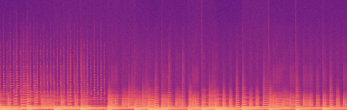
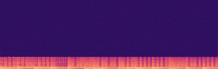
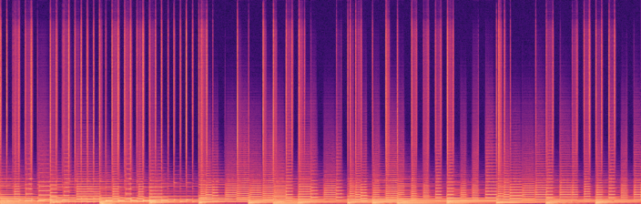
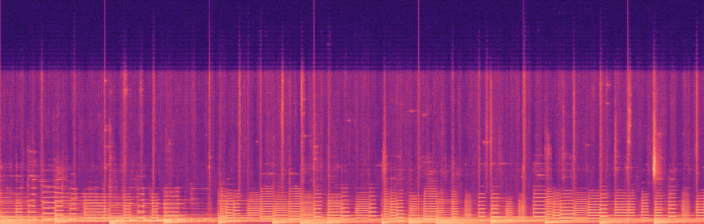
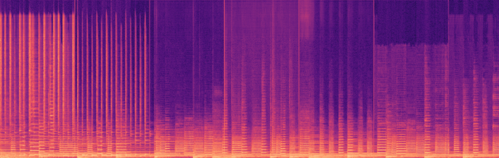
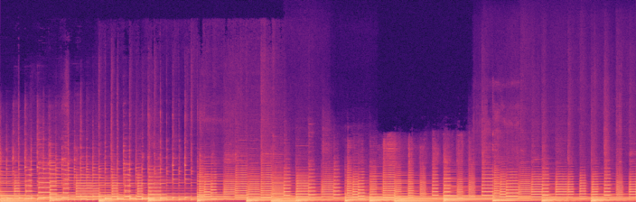
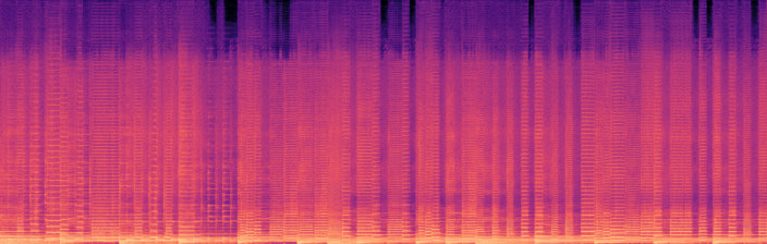
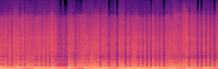
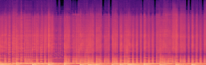
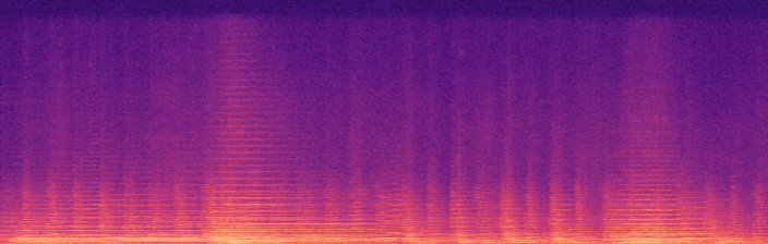
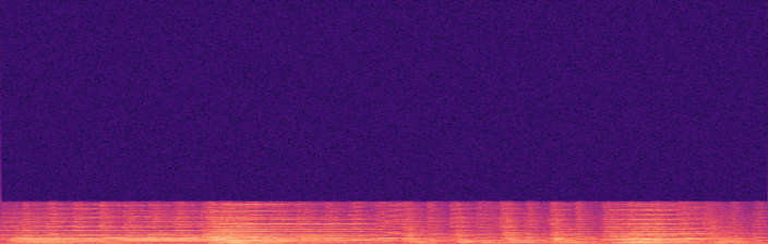
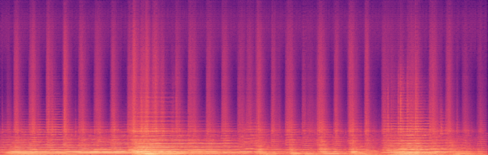
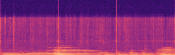
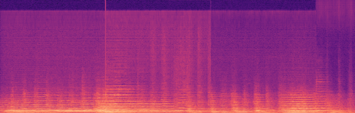
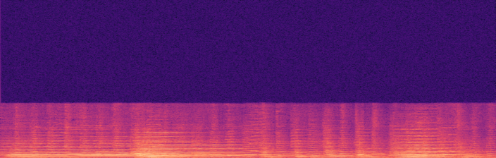
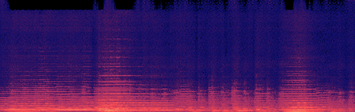
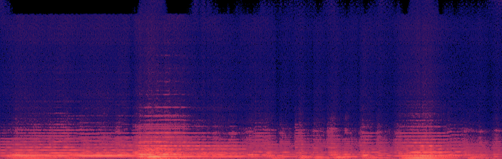
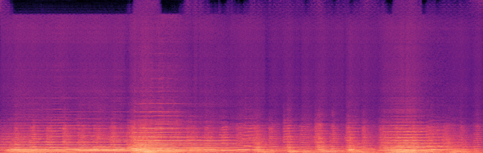
These matched examples combine clean, degraded, published baseline, and transport-based outputs for comparison by ear and by spectrogram. The transport outputs labeled Mean Shift and Local Mean are computed in the latent space of the Stable Audio Open VAE. Local Mean with Clean Lowband uses the same local-mean restoration, except that content below the 4 kHz cutoff is replaced by the original clean signal.
Audio example source. The listening examples on this page are taken from the A2SB demo website.
Five-Example Listening Summary
Mean raw-clean metrics aggregated over the five matched listening examples shown below: bwe_0, bwe_1, bwe_2, bwe_4, and bwe_5.